May 0, 2018
Timeseries Forecasting with Facebook Prophet and TM1/Planning Analytics

Welcome to the last part of the articles series about Data Science with TM1/Planning Analytics and Python. In Part 1 we loaded weather data from the NOOA web service into our TM1 cubes. In Part 2, by analyzing the data with Pandas and Ploty, we’ve learned that
- There are strong seasonal trends throughout the year
- Public Holidays and weekends have a negative impact on the bike shares
- Temperature and Bike shares are strongly correlated in every city.
- The intensity with which temperature affects the bike shares varies by city. Washington DC is the city that is least affected by the weather.
Before going any further, we recommend you to read these two articles:
- Part 1: Upload weather data from web service
- Part 2: Explore your TM1/Planning Analytics cube with Pandas and Ploty
Objective
In this article, we are going to explain how to use Facebook’s Prophet to create a two year demand forecast for bike sharing, based on four years of actuals from our TM1 cube.
Before we start with the implemenation let’s quickly discuss what Prophet is.
Prophet
The idea behind the prophet package is to decompose a time series of data into the following three components:
- Trends: these are non-periodic and systematic trends in the data,
- Seasonal effects: these are modelled as daily or yearly periodicities in the data (optionally also hourly), and
- Holidays / one-off effects: one-off effects for days like: Black Friday, Christmas, etc.
Based on our historic data, Prophet fits a model, where each of these components contribute additively to the observed time series. In other words, the number of bike shares on a given day is the sum of the trend component, the seasonal component and the one-off effects.
Step 1: Data Wranging
In the Part 2 of this series, we already loaded the actuals from the Bike Sharing cube into Python. We called the variable df_b.
Before we can use this data to fit our Prophet model, we must make sure we arrange the data in a correct format.
The dataframe that Prophet needs has two columns:
- ds: dates
- y: numeric values
We execute the following code to arrange our dataframe.
df_nyc = df_b[city].reset_index()df_nyc.rename(columns={'Date': 'ds', city: 'y'}, inplace=True)df_nyc.tail()We use the tail function on our dataframe (df_nyc) to display the last 5 rows of data:

Step 2: Fitting the model
Now that we have the data ready, and a high level understanding of the seasonal trends in our data, we are ready to fit our model!
First we need to instantiate Prophet. We are passing two arguments to the constructor of the Prophet model:
- The public holidays that we want Prophet to take into account
(they come from a TM1 cube through MDX. More details in the Jupyter notebook) - Whether or not Prophet should model intraday seasonality
m = Prophet(holidays = holidays, daily_seasonality=False)
Now we can fit our model, by executing the fit method on our model and passing the dataframe, that we arranged in step 1.
m.fit(df_nyc);
This is where Prophet is actually doing all the hard work, the curve-fitting.
Under the hood Prophet uses Stan to run the statistical calculations as fast as possible.
Step 3: Use Facebook’s Prophet to forecast the next 2 years
We can use the fitted Prophet model, to predict values for the future.
First we need to specify how many days we would like to forecast forward.
This code block creates a dataframe with the sized window of future dates.
future = m.make_future_dataframe(periods=365*2)
Then we use the predict function on our model. As the argument to that function, we pass the dataframe future.
forecast = m.predict(future)
Done!
The forecast is ready. Let’s look at what Prophet predicted !
We select the following columns on the dataframe and print out the last 5 records:
- ds (the date)
- yhat (the predicted value)
- yhat_lower (the lower bound of the confidence interval)
- yhat_upper (the upper bound of the confidence interval)
The following code is going to print the last 5 records:
forecast[['ds', 'yhat', 'yhat_lower', 'yhat_upper']].tail()

Step 4: Analysing the forecast
We can interrogate the model a bit to understand what it is doing. The best way to do this is to see how the model fits existing data and what the forecast looks like. This is shown in the plot below.
The black dots correspond to the historic number of bike shares each day (2014-2018). The dark blue line represents the estimated number of shares, projected with the fitted model.
The light blue lines correspond to the 80% confidence interval for the models predictions.
Judging visually, the model has done a good job of picking up the yearly seasonality and the overall trend. The forecast for 2019 and 2020 looks plausible!

To get an even further understanding of our fitted model, we can plot each of the model components. This is shown in the plot below.
In the top panel we see the linear growth term. This term contains changepoints (either determined independently by Prophet or preset by the user) so that the rate of growth is allowed to vary over time. The second panel shows the effect that public holidays have on our bike shares. The final two panels show the estimated yearly and weekly trends of the model:
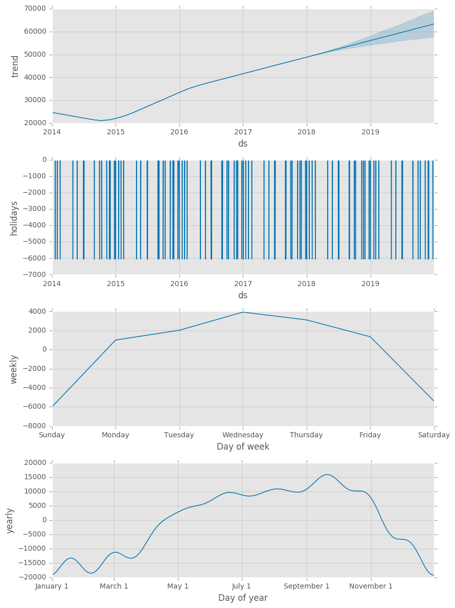
Conclusion on this analysis:
- An overall global trend of growth from 2015, that slowed down slightly after 2016.
- Public holidays lead to a fall in the usage of the bikes
- A strong weekly seasonality: Our bikes are used mostly during the week – presumably for commuting.
- A strong yearly seasonality with a peak in summer/ automn and a drop in winter.
Step 5: The last step is to send the data back to TM1
Before sending the data back to TM1, we need to rearrange the data so it matches the dimensions in our cube:
- Version: Prophet Forecast
- Date: date
- City: city
- Bike Shares Measures:
- Count for yhat
- Count Lower for yhat_lower
- Count Upper for yhat_upper
To rearrange the data for TM1 we execute the following code.
cells = {}for index, row in forecast.iterrows(): date = str(row['ds'])[0:10] cells['Prophet Forecast', date, city, 'Count'] = round(row['yhat']) cells['Prophet Forecast', date, city, 'Count Lower'] = round(row['yhat_lower']) cells['Prophet Forecast', date, city, 'Count Upper'] = round(row['yhat_upper'])Once our data set is ready, we use the TM1py function tm1.cubes.cells.write_values to send the data to our cube Bike Shares:
tm1.cubes.cells.write_values('Bike Shares', cells)Let’s check in the cubeview, years from 2014 to 2017 are actual data and the forecast starts in 2018:

See Prophet in action with Jupyter